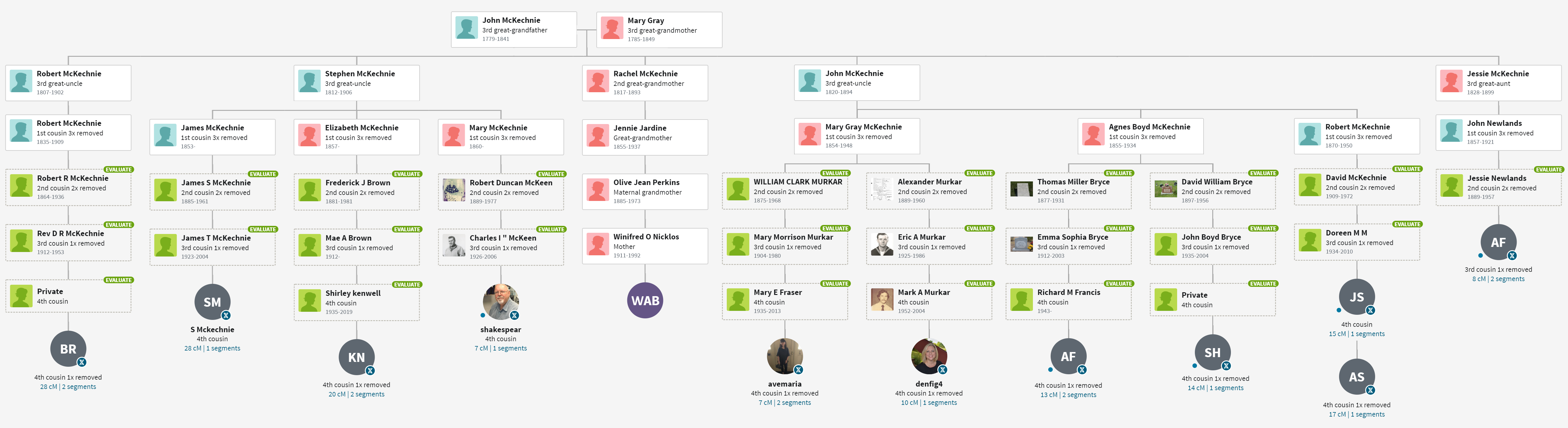
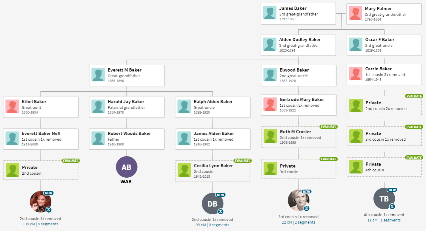
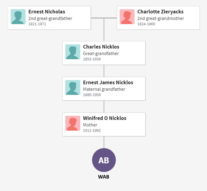
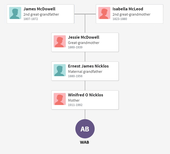
DNA results for my mother are in, so now it’s time to analyze the data. The goal is to validate and extend the lineage for that side of the family. So let’s start with the family tree, and show all the people who contributed their DNA to Mom, listed by her initals, WAB, in an attempt to preserve some small level of internet privacy. The DNA tested, called autosomal DNA, represents the mix of all your ancestors. It remains useful to at least the six generations shown below, even further.
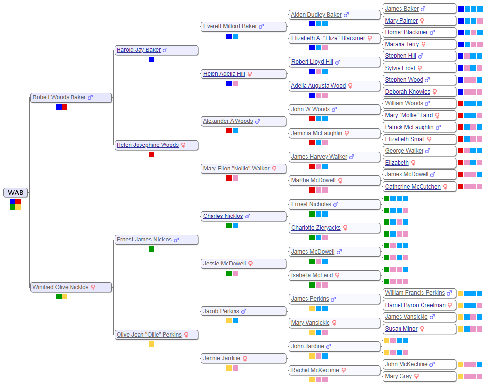
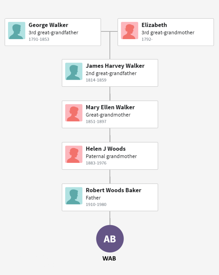
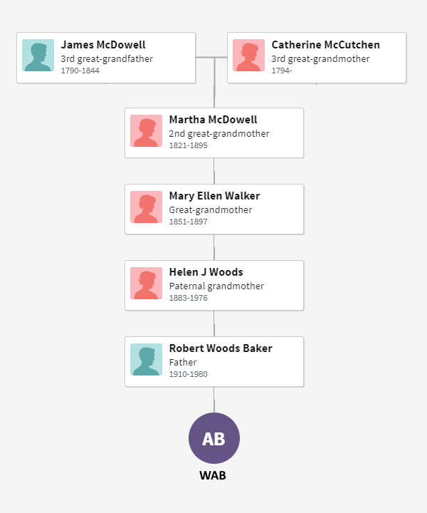
Look at the grandparents of WAB and you can define four distinct subgroups: Baker, Woods, Perkins and Nicklos. In DNA and geographic terms, each subgroup is quite unique. During the 1800’s, the Bakers lived primarily in New York, the Woodses lived in western Pennsylvania, the Perkinses settled Ontario emigrating from Nova Scotia and Scotland (Jardine), and the Nickloses immigrated to Canada from Scotland (McDowell) and Saxony, Germany (Nicklos). Since each subgroup is so distinct, it is useful to color code the four different subgroups with navy blue for Baker, red for Woods, yellow for Perkins and green for Nicklos, abbreviated N, R, Y and G respectively.
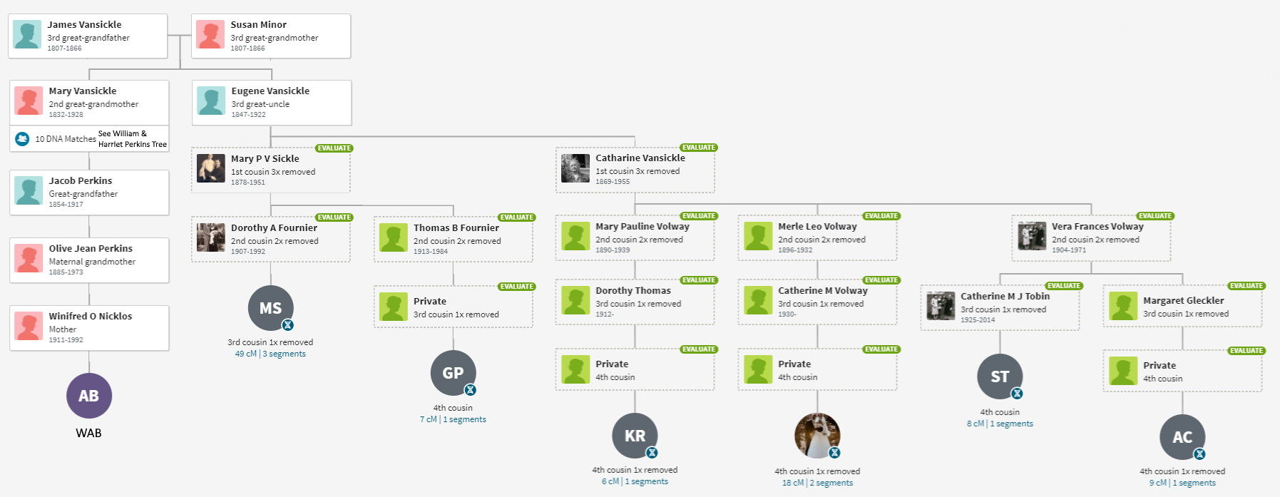
The use of subgroup names, while convenient, can be misleading. A Jardine, Vansickle, McKechnie, Creelman, Minor or Gray might feel a little slighted sitting in the Perkins subgroup. As an alternative, let me introduce generic light blue and pink color codes, abbreviated B & P, representing a father’s and mother’s DNA, respectively. Using this coding scheme, the sequence of YBP represents the DNA of Olive Perkins’s father’s mother, better known as Mary Vansickle. She, and all her brothers and sisters, as well as all their descendants, share the same common ancestor, James and Susan (Minor) Vansickle. Notice that color codes get longer with more distant relations.
DNA Matches
As a first pass, AncestryDNA shows everyone who shares DNA with you. The amount of shared DNA is measured in centimorgans (cM). It starts high and decreases rapidly with the generations. At some point, you share so little DNA that it’s possible that the match represents pure random chance, not a true relationship (a “false positive”). Per the lower right table, 30 cM represents a good conservative cut-off, giving about 95% confidence that the match is related to you. Later analysis will use a 20 cm threshold to look for additional matches. However, the table suggests that the risk of finding a false positive approaches 50%. Keep in mind that DNA results represent one part of a genealogy proof, which includes traditional evidence such as vital, probate and census records. While supporting documents are always needed, the need increases when using 20 cM DNA. WAB’s family tree is very important to our analysis because it contains references to that traditional supporting evidence.
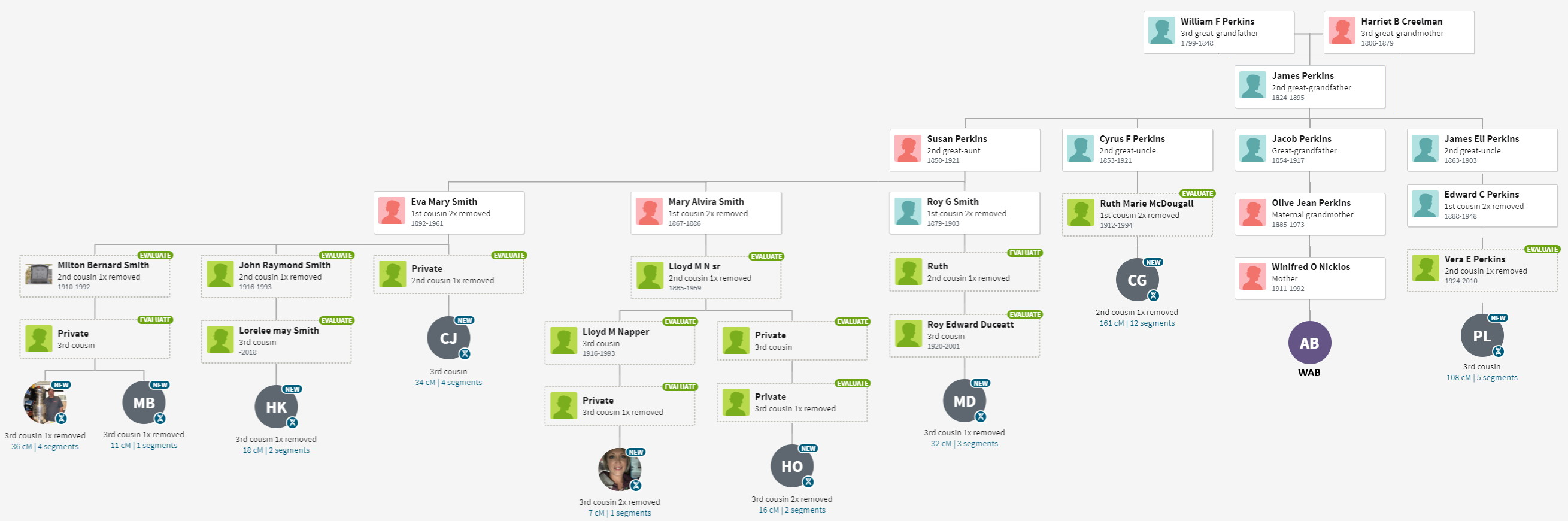
Scroll through the bottom left image from ancestryDNA to show the top DNA matches through “third cousin”. AncestryDNA will estimate the relationship based on the amount of shared DNA. Some users also provide family trees. Trees can be linked, unlinked or private. AncestryDNA will determine a “common ancestor” to linked, nonprivate trees. Each of the individuals is definitely related to WAB based on the large amount of shared DNA all of which exceed 90 cM.
| Confidence Score | Approximate amount of shared cM's | Likelihood of a single recent common ancestor |
|---|---|---|
| Extremely high | > 60 cMs | Virtually 100% |
| Very High | 45 - 60 cMs | About 99% |
| High | 30 - 45 cMs | About 95% |
| Good | 16 - 30 cMs | About 50% |
| Moderate | 6 - 16 cMs | 15 - 50% |
The Shared Match
So you share data with someone else, but what is the connection? More accurately: Who are the common ancestors? AncestryDNA has a very useful tool to help you identify the DNA that we share with another person called the “shared match”. Let’s say you are Person A. You select a person who shares DNA with you. Call them Person B. Shared matches shows all others who share DNA with Persons A & B.
The scrolling image to the right shows all DNA shared down to 20 cM with someone managed by MNeff. This person must be a close relative since they share 253 cM of DNA. Ethel (Baker) Neff, sister of our Harold J Baker, wrote a Baker family genealogy many years ago, likely making Everett and Helen (Hill) Baker our common ancestors. Color code-wise, MNeff is an N, and all the shared matches should also have an N. One would expect the shared matches to intersect with surnames like Baker, Hill, Blackmer, and Palmer, namely color codes like NB, NP, NBP and NBBP.
Determining a shared match involved some art mixed with the science. AncestryDNA uses a propriety computer algorithm to determine a shared match. Algorithms can be tricked, so a predicted match is fallible. A better technique would involve chromosome maps, the current gold standard for evaluating shared matches. AncestryDNA does not provide these maps citing privacy concerns. Yet, ancestryDNA has the the largest set of user submitted trees and DNA. Hope springs eternal that ancestryDNA changes its policy.
Tons of shared matches exist, making it tedious to analyze all of them. Fortunately, two tools can make this process much easier: ThruLines and Genetic Affairs.
ThruLines
ThruLines combines user-submitted trees along with DNA matches to group individuals. So two people can share very little DNA (well under 10 cM), but still show a match because their trees overlap. ThruLines can produce impressive trees, and has a lot of potential to expand the current tree. However, ThruLines has a bad reputation in the research community. It requires a family tree on AncestryDNA, some many of which perpetuate errors. Not surprisingly, misleading results continue to surface when you cross someone’s small, random DNA match and their flawed tree. AncestryDNA compounds the problem because they did not have system for fixing obvious errors.
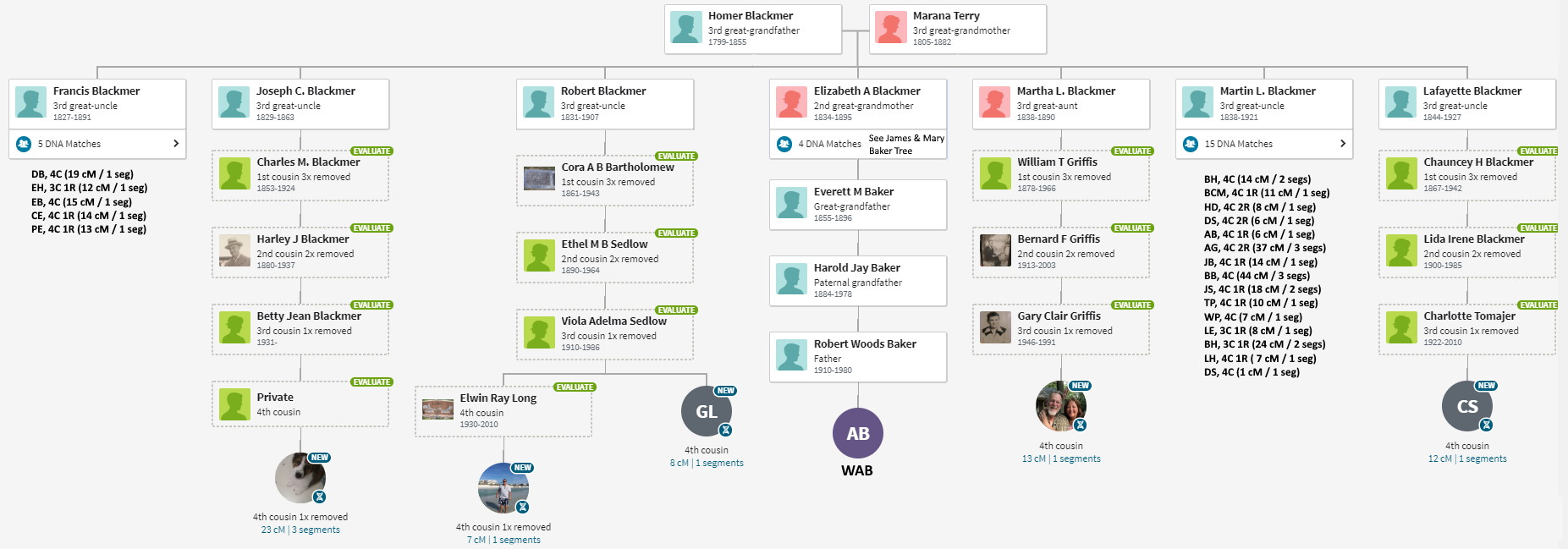
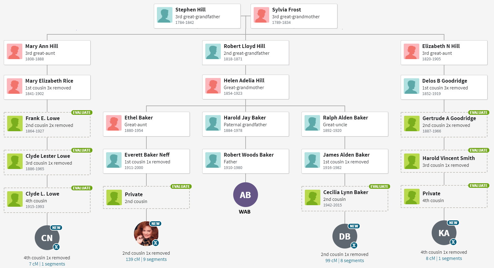
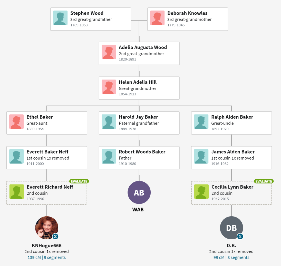
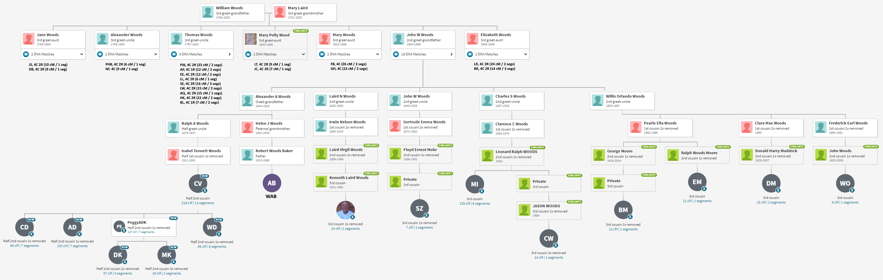
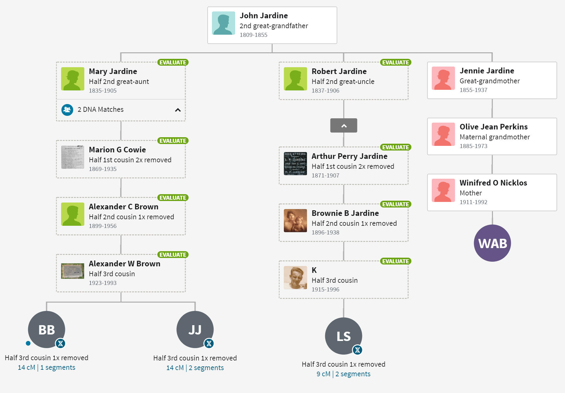
For me, ThruLines has proved useful because it allows me to analyze DNA under 20 cM. Below is a series of ThruLine charts for WAB, from James Baker to Mary Gray. Some trees have lots of matches, others not so much. Later I will use ThruLines to check some “what if” scenerios where you can postulate a relationship, and then see how people match.
Notice that these Thrulines cover a subset of available shared matches – those who have provided a useful tree. ThruLines do not get generated for matches who do not provide enough of a tree. Many times, I can fill in the gap and generate a similar chart. To differentiate them, allow me to modestly call them a “TrueLine” because the reader should have better confidence in their accuracy.
Genetic Affairs
This third-party utility forms a series of “clusters” from all the shared matches. In Mom’s case, the Baker family clusters would be very different than the Woods, Nicklos and Perkins clusters. No family trees are used to create the clusters. However, if you can identify one common ancestor, then everyone in that cluster should be related to that person. It’s a great way to examine the data. Click on the button below to see Genetic Affairs in action.
The drawing to the right shows clusters 1 and 2. Notice that the chart has perfect symmetry along the its diagonal axis (The information may be a little redundant, but the charts look fabulous). Cluster 1 has 12 members. The first member, C.V, shared DNA with the other 11. The second member, L.W., shares DNA with everyone but D.K. I have not, to date, paid any attention the relational pattern within a cluster. It’s pretty obvious that an entire family associated with PeggyADK has tested. Some Members (L.W…, MizCherie, and Susan Maddock) of cluster 1 share data with cluster 2, so the two clusters are somehow related.
How does Genetic Affairs decide when cluster 1 ends, and 2 begins? It’s magic. Actually, it’s another computer algorithm. As mentioned earlier, algorithms can be fooled and you will occasionally see misplacement of members into the wrong cluster.
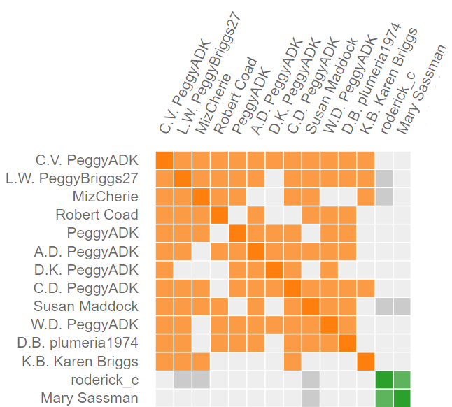
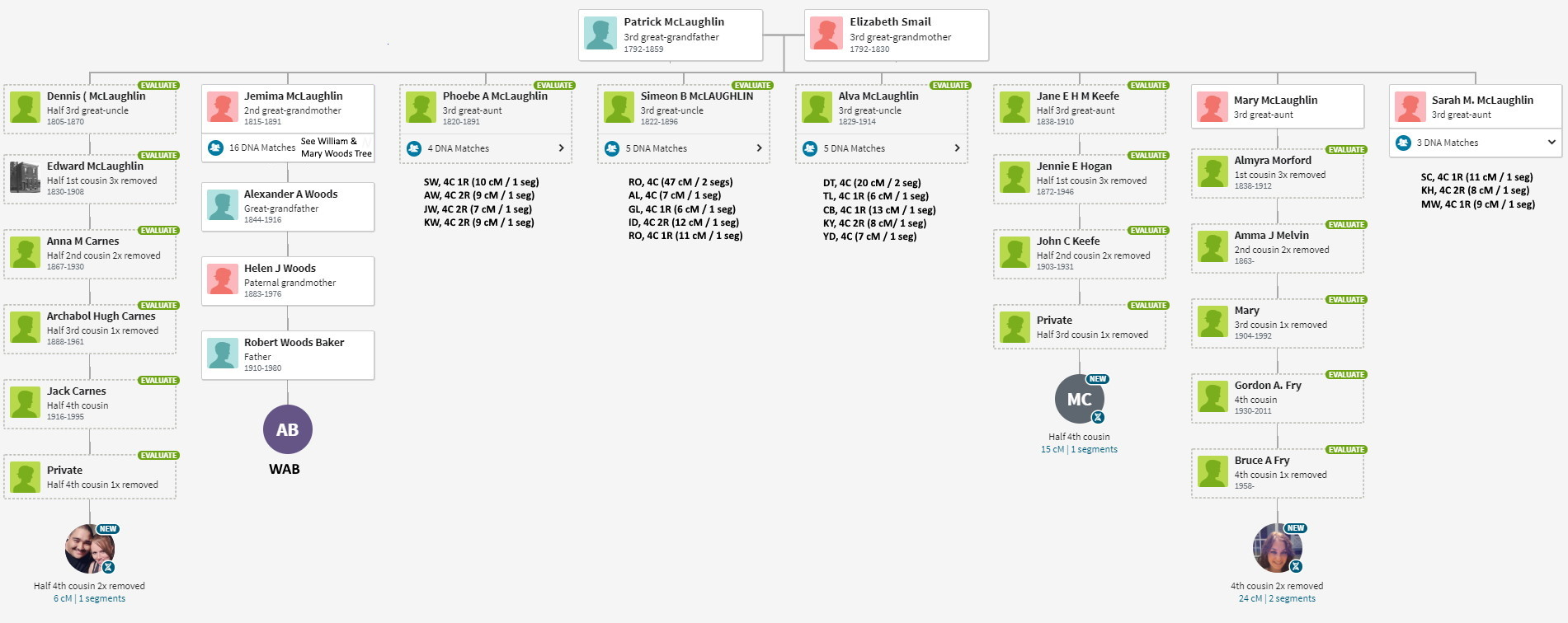
The cluster chart was further enhanced on the left side of the graph by showing the common ancestors, all identified from WAB’s Tree. For example, look for the sequence RBP in cluster 2 in the Woods subgroup. That member provided enough information that I learned that they descended from a brother of Jemima McLaughlin. Therefore our common ancestors are Patrick and Elizabeth (Smail) McLaughlin.
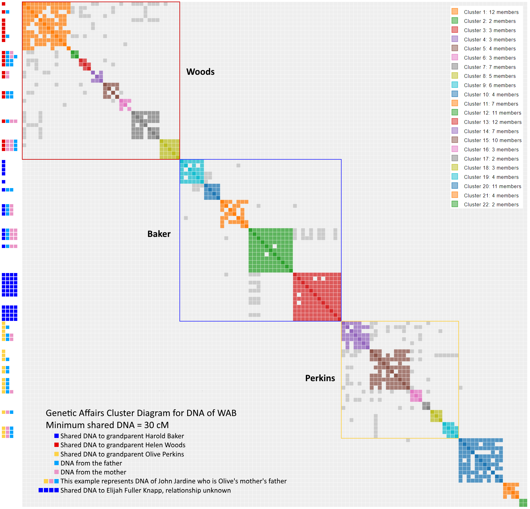
An obvious pattern emerges based on the WAB’s four grandparents where clusters 1 to 8 form a supercluster corresponding to the Woods subgroup, clusters 9 to 13 forms the Baker supercluster, clusters 14 to 19 forms the Perkins supercluster, and clusters 20 to 22 cannot yet be identified. Do not underestimate the significance of the various scattered gray dots because they suggest that two clusters are related. The exact supercluster boxes are subject to interpretation. For example, Perkins supercluster could have been included cluster 20 based on a single gray dot outside the yellow box. Overall, WAB’s DNA offers a textbook example of a “clean” Genetic Affairs cluster chart.
- The Woods supercluster is distinct from the Baker supercluster and the Perkins supercluster.
- Within each supercluster the most closely related descendant lies in the upper left quadrant; the least closely related is located bottom right. For example, the Woods supercluster starts at Cluster 1, color code R, and ends at cluster 8, a RPPB. Although Genetic Affairs behaves like it knows WAB’s tree, it simply orders the clusters by the amount of shared DNA. Cluster 1 shares the most DNA with WAB, Cluster 8 the least near the 30 cM threshold.
- The clusters within the superclusters show various common ancestors. In the Woods supercluster, Cluster 1 is a R, Cluster 2 is a RBP or RBPB, Cluster 4 is a RP, Cluster 5 is a RBB and cluster 8 is a RPPB. You can look up the various common ancestor on the tree above.
- No extraneous gray dots. The superclusters account for all of them (spoiler alert: I have since discovered that cluster 20 should be included with the Perkins supercluster).
Each cluster diagram is unique, and tells a slightly different story. What’s that NNNN sequence dominating cluster 13 of the Baker subgroup? I don’t know yet, but they all the members point to a guy named Elijah Fuller Knapp. Stay tuned for later essays focused on the each subgroup. Hopefully, I can answer the question by the time I write the article..
Conclusion
WAB’s DNA provides excellent understanding of her Baker, Woods and Perkins trees. While the Nicklos/McDowell lines remain missing, all is not lost. We have some good places to look, starting with the mystery clusters 20, 21 and 22. Also, Genetic Affairs listed 9 samples above the 30 cM threshold that are loners, and not part of any cluster. Results of these mystery matches will be left to the next article.