The last essay (DNA of WAB: Understanding the Gray) tried to explain the gray dots in the Genetic Affairs results at 20 cM on the Perkins subgroup. I concluded that the gray was a not necessarily a sign of endogamy or pedigree collapse, but should be embraced as a feature of an “ideal” tree. There is another aspect of low threshold cluster diagrams that needs to be discussed. Genetic Affairs has increased difficulty sorting the clusters as the minimum threshold drops from 30 to 20 cM. So in this essay, I want to describe the general problem at 20 cM and propose a solution. A more detailed discussion of the Woods family will wait for a future essay.
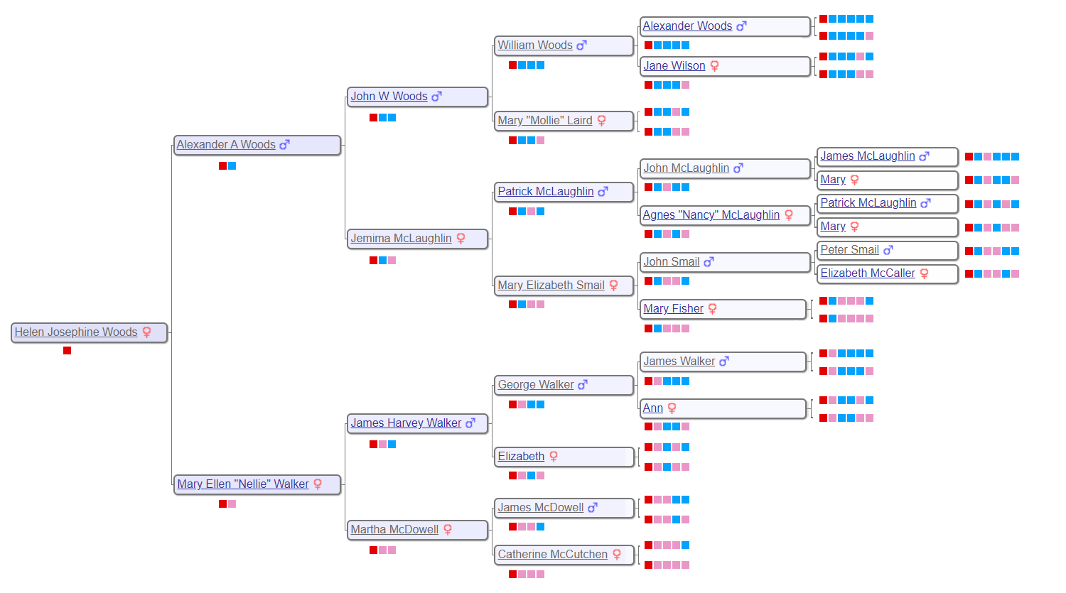
The process for creating the Woods results is similar to before. The six generation tree for Helen Woods is shown below, along with the portion of the 30 cM WAB Genetic Affairs cluster diagram that shows the Woods subgroup. The extend-a-cluster technique was utilized to create a 20 cM Woods cluster diagram. I then looked through all the shared matches to find as many common ancestors as possible, and added them to the diagram using the Red(R), Blue (B) and Pink (P) coding scheme.
Six Generation Family Tree for Helen Josephine Woods
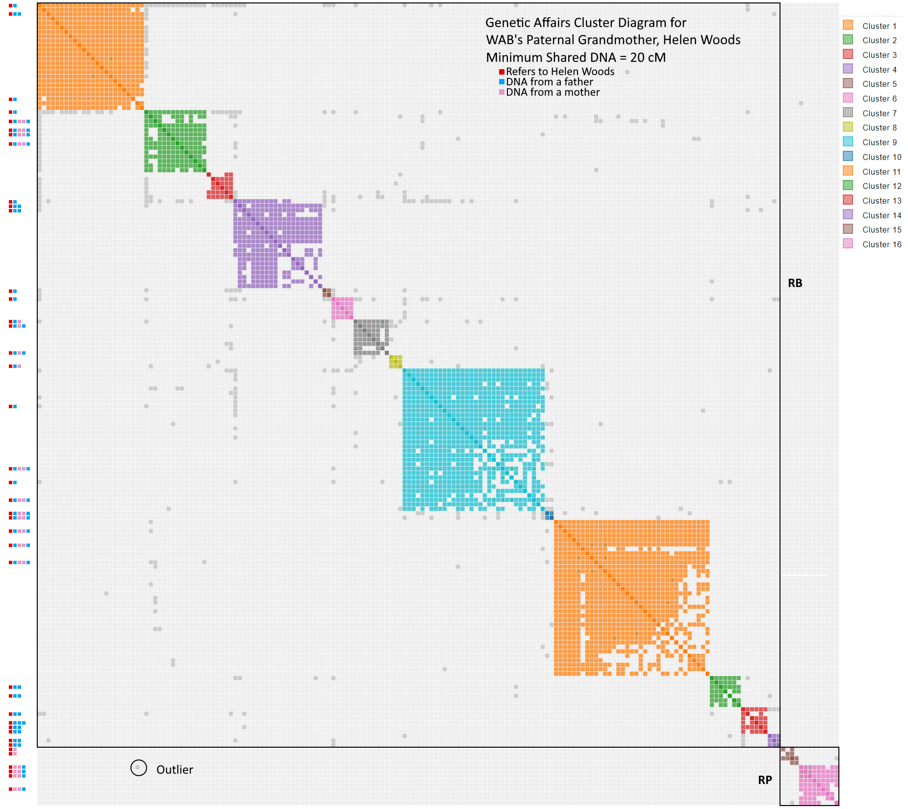
Initial WAB AutoCluster at 20 cM for the Woods Subgroup
How do you make sense of the cluster diagram? The cluster diagram clearly shows the differentiation between Helen’s father and mother, who are a RB and RP respectively. However, her father’s side, which dominates the diagram, is hopelessly mixed. Look how the shared matches with common ancestor RB get scattered across clusters 1, 2, 4, 5, 6 and 9. Fortunately, I can reapply my son’s algorithm to this plot and reassign the known shared matches. Here is the technique:
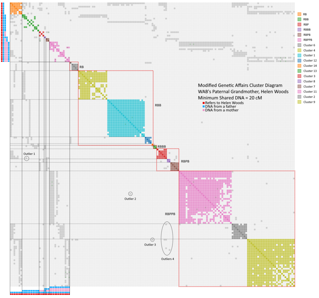
First, all the RP’s were turned off, because I need to focus on the RB results
The known tree results are put into unique clusters in the upper left corner. This created six reference clusters.
The remaining shared matches were kept in their previous clusters. Clusters 5 and 10 disappeared because they landed in the reference clusters.
By looking at the distributions of the gray dots, patterns emerged showing that certain clusters should be lumped together into superclusters.
Cluster 6 shares matches with reference RB and has one shared match with RBB. I am calling it a RB, where that first shared match should probably be moved to RBB. Or this whole cluster could be a RBB (there is a lot of art to this science).
Clusters 1, 4, 12 and 14 share matches with references RB and RBB. I am calling this supercluster a RBB
Cluster 13 shares matches with references RBB and RBBB, which would make it a RBBB.
Clusters 3, 7 and 8 share gray with references RB, RBP and RBPB making it a RBPB.
Clusters 2, 7 and 11 all share with references RB, RPB and RBPPB, making this supercluster a RBPPB.
All grays dots are explained by a normal tree except for the outliers noted below. Outlier 1 is a RBB-RBPB. Outliers 2 and 3 are RBB-RBPPB, and outliers in 4 are RBPB-RBPPB. The last group is perhaps the most interesting because they suggest the endogamy or pedigree collapse needed to raise the shared match level high enough to exceed 20 cM for very distant relatives.
Modified WAB AutoCluster at 20 cM for the Woods Subgroup - With Guide Lines
Congratulations if you have followed along this far. It is a little convoluted, but it is the only way I can make sense of the clusters generated by Genetic Affairs at this 20 cM level. Now, for example, I can focus my attention on the RBB supercluster in search of shared descendants to Mollie Laird who was a RBBP. Look below to see a clean version of the chart above without the guide lines.
What is going on here? In a previous life, I did some engineering, and this result seems like a classic “signal to noise” problem. It’s similar to listening to music on an airplane. To hear the song, you either need a lot of signal (crank the volume), eliminate the noise source (however, turning off the engines is a very bad idea) or add a filter to lessen the noise relative to the signal (think noise cancelling headphones). In our case, the signal is going down because the threshold is decreasing, and the collection of shared matches is kind of noisy. RBB and RBPPB appear to me to contain those nasty pseudoclusters that do not lead anywhere. They act as the genealogical equivalent to noise. As a result, the Genetic Affairs algorithm starts to struggle. However, all is not lost. The reference clusters acts as the filter to help separate from real matches from the noise.
Modified WAB AutoCluster at 20 cM for the Woods Subgroup - The Clean Version
What’s next? A lot of the problem stems from the way that ancestryDNA establishes a shared match. It seems to create these annoying pseudoclusters. Since I cannot use a chromosome map to study them, I need to find a way to identify them and filter them out. Next, it would be nice to use the extend-a-cluster technique in specific regions under the 20 cM limit. Some regions seem to be more free from pseudoclusters than others. Finally, and most importantly, I need to show that the modified graph was worth the time to create it by adding meaningful results to the tree.